Predicting Commercial Building Energy Costs: What the Data Shows
This was a university research project conducted at the University of Arizona in November 2025. It ended up becoming the foundation for building Forsa.
Predicting energy expenditures in commercial buildings
Introduction/Background:
Predicting total energy consumption within buildings is often one of the most challenging tasks regarding commercial buildings. When buyers purchase large commercial properties, they often lack information on the energy costs that the building will incur.
One of the biggest issues commercial real estate stakeholders have is the uncertainty around energy and utility costs, which is even more apparent in large scale buildings. Another important group is city officials, who need to know how a proposal development of a new building will demand energy and what impact it will have on the grid.
This econometric model attempts to estimate and implement a more accurate view of energy costs within a prospective commercial building. This model can be used to predict the energy consumption of buildings and, by extension, predict the operational energy costs of a building.
Proposed Models & Hypotheses:
Empirical model
ln(Energy Expenditure) = β0 + β1 ln(Sqft.) + β2Age + β3Region + β4City + β5Use + β6Cert + β7Renov + β8(Age × Cert1) + ε
Variable definitions
- Sqft. is a numeric variable that measures the total amount of square footage for the building. This variable is logged because it is not an apples-to-apples comparison; a logarithmic variable captures this far better.
- Age is a numeric variable that measures the age of the building.
- Region is a categorical variable that captures what region of the United States the building is in.
- City is a dummy variable which captures whether or not the building is located in a city.
- Use is a categorical variable which captures the primary function of the building—retail, office, industrial, multifamily, etc. This variable was originally named PBA (Principal Building Activity).
- Cert is a variable capturing green building or energy certification status for the property (as coded in the dataset).
- Renov is a binary variable that captures whether a building has completed a renovation since 2000.
- Age × Cert1 is an interaction variable which attempts to capture if green energy certifications offset building age.
- ε captures the unexplained noise and random variation within the model and is assumed to have zero conditional mean.
The hypothesis from this model is that sq footage, age, and use will be the three most important factors in predicting total energy expenditures for a commercial building. Having a positive effect and driving up total energy expenditures.
Data:
The dataset used in this project is a 2018 Commercial Building Energy Consumption Survey (CBECS). The report was compiled by the U.S. Energy Information Administration (EIA), a department of the U.S. Department of Energy. The survey estimates 5.9 million commercial buildings worth about $141 billion of energy expenditure. The process that the CBECS uses is a random sample survey, where every commercial building has a known chance of being selected. They collect information in-person and through a web survey.
Two key procedures were used in data cleaning and interpretation. The first task was renaming variables to be more interpretable. This was done by reading the codebook which is provided by CBECS. This spreadsheet includes a list of variable keys and a description of their meanings. The next step was renaming them in R. (E.g. PBA (Principal Building Activity) was renamed to Use, and others were also renamed). Second step was removing all variables that included blank or 0 variables, as they could have had a big impact on the model.
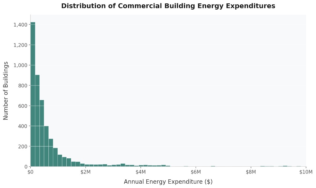
Another step was generating a histogram to get a visual idea of the data:
Estimation Method:
OLS (Ordinary Least Squares) was used which minimizes the sum of squared residuals. The log-linear specification allows coefficients to be interpreted as percentage changes. Additionally, hold-out validation was used to split the data and test.
Hypothesis Test
Two hypothesis tests were run, with 95% and 99% confidence intervals.
The 95% CI with 6356 degrees of freedom yielded a t-statistic of 34.768 a p-value of <2.2e-16 and the interval from 292,065-326,968. With a sample mean of 309,517. Therefore, because our p-value < 0.05 we reject the null and can conclude that the mean energy expenditure lies between $292,065-$326,968 with 95% confidence.
Figure 1 95% Hypothesis Test:
One Sample t-test

data:  EnData$MFEXP
t = 34.768, df = 6356, p-value < 2.2e-16
alternative hypothesis: true mean is not equal to 0
95 percent confidence interval:
 292065.2 326968.8
sample estimates:
mean of x
 309517
The 99% CI with 6356 degrees of freedom yielded a t-statistic of 34.765 and a p-value of <2.2e-16. We get an interval of 286,578-332,455 with a sample mean of 309,517. Therefore, we can conclude that the sample mean lies between our interval with 99% confidence, and reject the null hypothesis.
Figure 2 99% Hypothesis Test:
One Sample t-test

data:  EnData$MFEXP
t = 34.765, df = 6356, p-value < 2.2e-16
alternative hypothesis: true mean is not equal to 20
99 percent confidence interval:
 286578.9 332455.1
sample estimates:
mean of x
 309517
Estimation Results:
From our regression output, there are some notable findings. A 1% increase in shift increases energy expenditure by 0.96%, which is almost proportional. Inconsistent with assumptions, older buildings consume slightly (marginally) less energy each year. Buildings in city consume 17% more on energy, and consistent with assumptions building expenditure vary drastically by use.
Figure 3: Regression output
Call:
lm(formula = ln_energy_exp ~ ln_sqft + age + region_south + city + use_category + cert1 + cert2 + RENOV + age:cert1, data = EnData_clean)
Residuals:
    Min      1Q  Median      3Q      Max
-4.9189 -0.3252  0.0220  0.3493  2.2950
Coefficients:
(1 not defined because of singularities)
| Estimate | Std. Error | t value | Pr(>|t|) | ||
|---|---|---|---|---|---|
| (Intercept) | -0.6319143 | 0.1241971 | -5.088 | 3.81e-07 | *** |
| ln_sqft | 0.9564285 | 0.0077999 | 122.621 | < 2e-16 | *** |
| age | -0.0011626 | 0.0006338 | -1.834 | 0.0667 | . |
| region_south | -0.1156758 | 0.0203703 | -5.679 | 1.47e-08 | *** |
| city | 0.1737853 | 0.0195935 | 8.870 | < 2e-16 | *** |
| use_category2 | 1.3389687 | 0.0899239 | 14.890 | < 2e-16 | *** |
| use_category4 | 2.1353494 | 0.1222149 | 17.472 | < 2e-16 | *** |
| use_category5 | 0.5102079 | 0.0948431 | 5.379 | 7.96e-08 | *** |
| use_category6 | 2.5653323 | 0.1277892 | 20.075 | < 2e-16 | *** |
| use_category7 | 1.3121556 | 0.1184008 | 11.082 | < 2e-16 | *** |
| use_category8 | 1.5677211 | 0.1028560 | 15.242 | < 2e-16 | *** |
| use_category11 | 1.9459635 | 0.2340417 | 8.315 | < 2e-16 | *** |
| use_category12 | 0.6261621 | 0.0998493 | 6.271 | 4.02e-10 | *** |
| use_category13 | 1.3225944 | 0.0946188 | 13.978 | < 2e-16 | *** |
| use_category14 | 1.0172300 | 0.0912476 | 11.148 | < 2e-16 | *** |
| use_category15 | 2.5727412 | 0.1057482 | 24.329 | < 2e-16 | *** |
| use_category16 | 2.0693986 | 0.0966339 | 21.415 | < 2e-16 | *** |
| use_category17 | 1.6607350 | 0.1136208 | 14.616 | < 2e-16 | *** |
| use_category18 | 1.3934357 | 0.0942091 | 14.791 | < 2e-16 | *** |
| use_category23 | 1.7126281 | 0.1051474 | 16.288 | < 2e-16 | *** |
| use_category24 | 0.8140500 | 0.1389420 | 5.859 | 5.09e-09 | *** |
| use_category25 | 1.3827386 | 0.0966065 | 14.313 | < 2e-16 | *** |
| use_category26 | 1.0816734 | 0.1018339 | 10.622 | < 2e-16 | *** |
| use_category91 | 2.1320920 | 0.1409322 | 15.128 | < 2e-16 | *** |
| cert1 | 0.3061775 | 0.0449298 | 6.815 | 1.11e-11 | *** |
| cert2 | 0.0332065 | 0.0232333 | 1.429 | 0.1530 | |
| RENOV | NA | NA | NA | NA | |
| age:cert1 | -0.0012474 | 0.0008528 | -1.463 | 0.1436 |
Signif. codes: 0 ‘***’ 0.001 ‘**’ 0.01 ‘*’ 0.05 ‘.’ 0.1 ‘ ’ 1
Model diagnostics
Our Adjusted R-Squared is 0.90. This model explains 90% of the variation in the dataset. Which is impressive. F-Statistic of 1344 (p<2.2e-16) meaning the model is highly significant. Our residual Standard Error: 0.5731 on 3515 degrees of freedom. A second model was also used which removed variables City, cert1, age, and city.
Figure 4: Model comparison output metrics
| Reduced model | Original model | |
|---|---|---|
| Observations | 3,542 | 3,542 |
| R2 | 0.903 | 0.909 |
| Adjusted R2 | 0.903 | 0.908 |
| Residual std. error | 0.589 (df = 3519) | 0.573 (df = 3515) |
| F statistic | 1,495.672*** (df = 22; 3519) | 1,343.693*** (df = 26; 3515) |
* p < 0.1; ** p < 0.05; *** p < 0.01
The first column is the first column (reduced) model, and second is the original. The original model had a higher adjusted R2 and lower residual Std. Error and thus, was selected.
Hold-out validation and Holt exponential smoothing
Hold-Out Method was performed using holt exponential smoothing. The optimized model performed better than the user model, With lower ME, RMSE, and MAE in the test set. The user model output indicates overfitting of the data.
Figure 5: Cross-validation error metrics
accuracy(forecast_user, actual_valid)
| ME | RMSE | MAE | MPE | MAPE | MASE | ACF1 | |
|---|---|---|---|---|---|---|---|
| Training set | −0.002564464 | 2.087811 | 1.688920 | −3.03182 | 15.69394 | 0.7806671 | −0.09365676 |
| Test set | 5.814841792 | 6.126311 | 5.814842 | 48.53442 | 48.53442 | 2.6877863 | NA |
accuracy(forecast_cmp, actual_valid)
| ME | RMSE | MAE | MPE | MAPE | MASE | ACF1 | |
|---|---|---|---|---|---|---|---|
| Training set | 0.001501282 | 1.875656 | 1.523166 | −3.00339 | 14.26933 | 0.7040510 | −0.02505734 |
| Test set | 0.008431686 | 1.920387 | 1.586933 | −3.06598 | 14.82865 | 0.7335257 | NA |
Conclusion/Implications:
This model and research provide an accurate basis for assessing building energy consumption. The framework can be used by a range of stakeholders who need to evaluate or predict energy use from observable building characteristics.
Still, there are three major limitations to keep in view. First, CBECS 2018 is a single snapshot; the nature of building energy performance has shifted since then, and many assets have become more efficient through operations, retrofits, and code cycles, so the coefficients are anchored in a past market regime. Second, several inputs are deliberately coarse: the renovation variable treats all renovations alike, the city indicator compresses heterogeneous urban contexts, and the certification coding does not capture every major green program a building might hold. Third, endogeneity and omitted-variable bias can distort inference—factors outside the survey (management quality, metering depth, unobserved capital plans) can influence both the regressors and the error term—so results should be paired with domain judgment and refreshed data when stakes are high.
References:
- BrainBox AI. “Mastering Building Energy Efficiency: EUI and Energy Consumption.” Brainboxai.com, Brainbox AI, 17 July 2024, https://brainboxai.com/en/articles/mastering-building-energy-efficiency-eui-and-energy-consumption.
- Bourdeau, Mathieu, et al. “Modeling and Forecasting Building Energy Consumption: A Review of Data-Driven Techniques.” Sustainable Cities and Society, vol. 48, July 2019, p. 101533, https://doi.org/10.1016/j.scs.2019.101533. Accessed 5 Feb. 2022.
- “Building Energy Use.” U.S. General Services Administration, 2023, https://www.gsa.gov/governmentwide-initiatives/federal-highperformance-buildings/highperformance-building-clearinghouse/energy/building-energy-use.
- EIA. “Energy Information Administration (EIA)—Commercial Buildings Energy Consumption Survey (CBECS).” Eia.gov, 2016, https://www.eia.gov/consumption/commercial/.
- “How Much Energy Is Consumed in U.S. Residential and Commercial Buildings?—FAQ—U.S. Energy Information Administration (EIA).” Eia.gov, 2016, https://www.eia.gov/tools/faqs/faq.php?id=86&t=1.